Understanding Regression in Machine Learning: Concepts, Algorithms, and Performance Metrics

Regression is one of the foundational techniques in machine learning, used when the goal is to predict a continuous numeric value based on one or more input features. Whether you’re estimating real estate prices, forecasting demand, or predicting crop yields, regression models help make informed, data-driven predictions.

This article breaks down the essentials of regression in machine learning—including the workflow, common algorithms, model adjustment strategies, and most importantly, how to evaluate model performance using appropriate metrics.

What Is Regression?

Regression models estimate the relationship between independent variables (features) and a dependent variable (target). The output is a continuous value, which distinguishes regression from classification (which predicts discrete categories).

Examples of regression tasks:

• Predicting housing prices based on area, location, and number of rooms.
• Estimating rainfall from atmospheric data.
• Forecasting energy consumption from historical usage and temperature patterns.

The Regression Workflow

1. Data Splitting
   • Split your dataset into a training set (typically 70–80%) and a validation/test set (20–30%).
   • The model is trained on the training set and evaluated on the validation set to test its generalizability.
2. Model Fitting
   • Choose and apply a regression algorithm. This step involves learning the best-fit parameters that minimize prediction error.
   • Algorithms may include Linear Regression, Polynomial Regression, Ridge, Lasso, or Bayesian Regression, depending on the complexity and nature of the data.
3. Prediction
   • Once trained, the model is used to predict outcomes on the validation data. These predictions are then compared with actual target values.
4. Evaluation
   • Assess how well the model performs using quantitative metrics. This helps determine whether to improve the model through iteration or finalize it for deployment.

Model Adjustment Techniques

Improving a regression model often requires a series of thoughtful changes:

• Feature Engineering
  • Add, remove, or transform input features. For example, if elevation does not influence crop yield significantly, it might be removed. Conversely, adding pest population data might improve accuracy.
• Algorithm Selection
  • Test different regression algorithms. If a linear model underfits the data, switching to Polynomial Regression might capture more complex patterns.
• Hyperparameter Tuning
  • Adjust parameters such as regularization strength in Ridge/Lasso Regression or degree of the polynomial in Polynomial Regression. Grid search and cross-validation help automate this process.

Common Regression Algorithms

• Linear Regression
  • Assumes a straight-line relationship between input variables and output.
  • Simple and interpretable; performs well when data has linear trends.
• Polynomial Regression
  • Extends linear regression by adding higher-degree terms (e.g., x², x³).
  • Useful for capturing curved relationships but more prone to overfitting if the degree is too high.
• Ridge and Lasso Regression
  • Both are regularized versions of linear regression that penalize large coefficients.
  • Ridge uses L2 penalty (squared coefficients), Lasso uses L1 (absolute values).
  • They reduce overfitting, especially when dealing with multicollinearity or many features.
• Bayesian Regression
  • Introduces probability distributions for the model parameters, giving not just point estimates but distributions.
  • Good for scenarios where uncertainty estimation is crucial.

Performance Metrics for Regression

Evaluating regression models is more than just checking how close predictions are to the actual values. The following metrics help you assess both the accuracy and behavior of your model:

1. Mean Absolute Error (MAE)

• Definition: The average of the absolute differences between predicted and actual values.
• Formula:

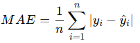
• Use: Easy to interpret, gives equal weight to all errors.
• Limitation: Doesn’t heavily penalize large errors.

2. Mean Squared Error (MSE)

• Definition: The average of the squares of the errors.
• Formula:

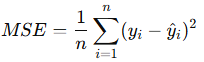
• Use: Penalizes large errors more than MAE, which is useful when large errors are particularly bad.
• Limitation: Units are squared; less intuitive for interpretation.

3. Root Mean Squared Error (RMSE)

• Definition: The square root of the MSE.
• Formula:

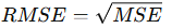
• Use: Returns the error to the original unit of measurement, making it more interpretable.
• Note: Like MSE, it penalizes larger errors more than smaller ones.

4. R² (Coefficient of Determination)

• Definition: Measures the proportion of variance in the target variable explained by the model.
• Formula:

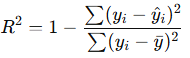
• Range: 0 to 1 (can be negative if model performs worse than predicting the mean).
• Interpretation:
  • R² = 1: Perfect prediction.
  • R² = 0: Model predicts no better than the mean.
  • R² < 0: Model is worse than predicting the mean.

Tip: Use multiple metrics in combination. For instance, a model may have a low RMSE but a poor R² score if it fails to generalize.

Final Thoughts

Regression is a powerful tool for any data scientist or machine learning practitioner. However, building a reliable regression model goes beyond choosing an algorithm—it requires thoughtful preprocessing, iterative adjustments, and a deep understanding of evaluation metrics. The right combination of features, model type, and tuning can significantly improve predictive performance.

Sample Regression Workflow code in python

import numpy as np
import pandas as pd
from sklearn.datasets import fetch_my_data
from sklearn.model_selection import train_test_split
from sklearn.linear_model import LinearRegression
from sklearn.metrics import mean_absolute_error, mean_squared_error, r2_score
import matplotlib.pyplot as plt

# 1. Load dataset
data = fetch_my_data()
X = pd.DataFrame(data.data, columns=data.feature_names)
y = data.target

# 2. Split data into training and validation sets
X_train, X_valid, y_train, y_valid = train_test_split(X, y, test_size=0.2, random_state=42)

# 3. Train the regression model
model = LinearRegression()
model.fit(X_train, y_train)

# 4. Predict on validation set
y_pred = model.predict(X_valid)

# 5. Evaluate performance
mae = mean_absolute_error(y_valid, y_pred)
mse = mean_squared_error(y_valid, y_pred)
rmse = np.sqrt(mse)
r2 = r2_score(y_valid, y_pred)

print("Performance Metrics:")
print(f"Mean Absolute Error (MAE): {mae:.4f}")
print(f"Mean Squared Error (MSE): {mse:.4f}")
print(f"Root Mean Squared Error (RMSE): {rmse:.4f}")
print(f"R² Score: {r2:.4f}")

# 6. Optional: Plot predictions vs actual values
plt.figure(figsize=(8, 6))
plt.scatter(y_valid, y_pred, alpha=0.4)
plt.plot([min(y_valid), max(y_valid)], [min(y_valid), max(y_valid)], color='red')
plt.xlabel("Actual Median House Value")
plt.ylabel("Predicted Median House Value")
plt.title("Predicted vs Actual Values")
plt.grid(True)
plt.tight_layout()
plt.show()