Binary classification is a fundamental task in machine learning where the goal is to categorize data into one of two classes. Whether predicting disease presence, detecting fraud, or classifying emails as spam or not, binary classification lies at the core of many real-world AI applications.
Let’s look at the principles of binary classification, commonly used algorithms, how models make predictions, and how to evaluate their effectiveness using key performance metrics.
What Is Binary Classification?
Binary classification is a supervised learning approach, meaning the training data includes both input features (X) and a target label (y). The target variable takes on only two possible values, usually represented as 0 and 1, or negative and positive, depending on the context.
Examples of binary classification problems:
- Is an email spam or not?
- Will a customer default on a loan: yes or no?
- Is a tumor malignant or benign?
- Does a patient have diabetes based on lab data?
How Binary Classification Works
A typical binary classification model learns patterns from training data to predict the probability that a given input belongs to the positive class (usually labeled as 1).
Prediction and Thresholding
- The model outputs a probability between 0 and 1.
- A threshold (commonly 0.5) is applied to this probability to make the final classification.
- If probability ≥ 0.5 → class 1 (positive)
- If probability < 0.5 → class 0 (negative)
The threshold can be adjusted depending on the importance of false positives vs false negatives (e.g., in medical diagnosis).
Common Algorithms for Binary Classification
Each algorithm has its strengths and ideal use cases. Here are some of the most popular binary classification methods:
🔹 Logistic Regression
- A linear model that applies the sigmoid function to map predictions to probabilities.
- Interpretable and efficient; good for baseline models and linearly separable data.
🔹 Decision Tree
- A tree-based model that splits data based on feature values.
- Handles nonlinear data well but can overfit without pruning.
🔹 Random Forest
- An ensemble of decision trees trained on random subsets of data and features.
- Improves generalization and reduces overfitting.
🔹 Support Vector Machine (SVM)
- Finds the optimal hyperplane that separates classes with the largest margin.
- Effective for high-dimensional spaces and cases where classes are not linearly separable (with kernel trick).
Performance Evaluation: Beyond Accuracy
Evaluating a binary classifier requires more than simply checking how often it gets predictions right. Let’s break down the key metrics used to measure performance.
Confusion Matrix
A 2×2 matrix that summarizes predictions:
| Predicted Positive | Predicted Negative | |
|---|---|---|
| Actual Positive | TP (True Positive) | FN (False Negative) |
| Actual Negative | FP (False Positive) | TN (True Negative) |
Each element of the confusion matrix has a specific meaning:
- TP: Model correctly predicted positive.
- TN: Model correctly predicted negative.
- FP: Model predicted positive incorrectly (false alarm).
- FN: Model missed a positive case (false negative).
Accuracy
- Measures overall correctness of the model.
- Formula:
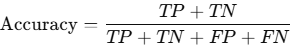
- Limitation: Can be misleading in imbalanced datasets (e.g., 95% negative class).
Precision
- Measures the quality of positive predictions.
- Formula:
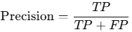
- High precision means few false positives.
Recall (Sensitivity or True Positive Rate)
- Measures the model’s ability to identify actual positives.
- Formula:
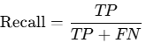
- High recall means few false negatives, which is crucial in medical or safety-related tasks.
F1-Score
- Combines precision and recall into a single metric.
- Formula:
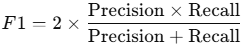
- Use: When you want a balance between precision and recall, especially in uneven class distributions.
📈 AUC – ROC Curve (Area Under the Curve)
- Plots True Positive Rate (Recall) vs False Positive Rate at various thresholds.
- AUC measures the model’s ability to distinguish between classes:
- AUC = 1.0 → Perfect classifier.
- AUC = 0.5 → Model is guessing randomly.
- Why it matters: AUC is threshold-independent, giving a broader view of model performance.
Example: Predicting Diabetes
Let’s say you’re building a model to predict whether a patient has diabetes using features like:
- BMI
- Age
- Cholesterol levels
- Blood pressure
If your model predicts a 0.84 probability of diabetes for a patient and your threshold is 0.5, you classify the patient as positive (has diabetes).
After evaluating the model on a test set:
- You find that precision is high but recall is low → The model rarely mislabels negatives as positives, but misses many true cases of diabetes.
- You might choose to lower the threshold to improve recall.
Final Thoughts
Binary classification is essential to modern machine learning systems. While it’s tempting to focus on accuracy, a nuanced view of other metrics like precision, recall, F1, and AUC ensures a more reliable and application-aware evaluation of model performance.
Whether you’re detecting disease, approving loans, or screening emails, a carefully tuned binary classifier can make powerful, high-stakes decisions—provided it’s evaluated and adjusted using the right metrics.
Python Code for Binary Classification
Library:
pip install pandas scikit-learn matplotlib seabornFull Code:
import pandas as pd
import numpy as np
from sklearn.model_selection import train_test_split
from sklearn.linear_model import LogisticRegression
from sklearn.metrics import (
    confusion_matrix,
    accuracy_score,
    precision_score,
    recall_score,
    f1_score,
    roc_auc_score,
    roc_curve,
)
import seaborn as sns
import matplotlib.pyplot as plt

# 1. Load dataset (downloaded from UCI repository or Kaggle)
url = "https://raw.githubusercontent.com/jbrownlee/Datasets/master/pima-indians-diabetes.data.csv"
columns = [
    "Pregnancies", "Glucose", "BloodPressure", "SkinThickness",
    "Insulin", "BMI", "DiabetesPedigreeFunction", "Age", "Outcome"
]
df = pd.read_csv(url, header=None, names=columns)

# 2. Features and target
X = df.drop("Outcome", axis=1)
y = df["Outcome"]

# 3. Split data into training and test sets
X_train, X_test, y_train, y_test = train_test_split(
    X, y, test_size=0.2, random_state=42, stratify=y
)

# 4. Train Logistic Regression model
model = LogisticRegression(max_iter=1000)
model.fit(X_train, y_train)

# 5. Make predictions
y_pred = model.predict(X_test)
y_prob = model.predict_proba(X_test)[:, 1]  # probabilities for ROC

# 6. Evaluate performance
conf_matrix = confusion_matrix(y_test, y_pred)
accuracy = accuracy_score(y_test, y_pred)
precision = precision_score(y_test, y_pred)
recall = recall_score(y_test, y_pred)
f1 = f1_score(y_test, y_pred)
auc = roc_auc_score(y_test, y_prob)

# 7. Print metrics
print("📊 Evaluation Metrics:")
print(f"Accuracy  : {accuracy:.4f}")
print(f"Precision : {precision:.4f}")
print(f"Recall    : {recall:.4f}")
print(f"F1-score  : {f1:.4f}")
print(f"AUC       : {auc:.4f}")

# 8. Visualize Confusion Matrix
plt.figure(figsize=(6, 4))
sns.heatmap(conf_matrix, annot=True, fmt="d", cmap="Blues", xticklabels=["No", "Yes"], yticklabels=["No", "Yes"])
plt.xlabel("Predicted")
plt.ylabel("Actual")
plt.title("Confusion Matrix")
plt.show()

# 9. ROC Curve
fpr, tpr, thresholds = roc_curve(y_test, y_prob)
plt.figure(figsize=(6, 4))
plt.plot(fpr, tpr, label=f"AUC = {auc:.2f}")
plt.plot([0, 1], [0, 1], linestyle='--', color='gray')
plt.xlabel("False Positive Rate")
plt.ylabel("True Positive Rate")
plt.title("ROC Curve")
plt.legend()
plt.grid(True)
plt.show()
Output:
Evaluation Metrics:
Accuracy : 0.7662
Precision : 0.7200
Recall : 0.5909
F1-score : 0.6486
AUC : 0.8240